
I trained a reinforcement learning model to play ‘Threes!’, a deceptively simple sliding puzzle game.
The result is a lightweight agent that can make instant decisions while retaining performance rivaling expert players. The AI can make about 100 moves or more per second — far faster than humans and even the best other ‘Threes’ agents (100x faster than the best agent) — and it can run locally on any machine. Try it out for yourself on GitHub.
Reinforcement learning is a subset of machine learning that specializes in domains requiring fast, effective decisions. It opens the door to cheaper, real-time systems that can navigate noisy or complex environments without massive amounts of training data.
Most strong game-playing systems rely on search techniques such as Expectimax or Monte Carlo Tree Search (MCTS) to evaluate future states. In contrast, this model learns a direct policy with little overhead: given the current board, choose the next move.
This trades off some optimality for speed and scalability, making it closer to how machine learning systems are deployed in real-world environments where lookahead (simulating outcomes) is expensive or infeasible.
For business leaders, the takeaway is less about solving a puzzle game and more about RL applications. This project demonstrates that specialized methods can be used to make fast, effective decisions in challenging environments without relying on heavy computation or complex simulation — a trade-off that matters in real-world operations.
In areas like supply chain routing or financial trading, decisions often need to be made instantly and at scale. When companies need to make actions instead of classifications, a lightweight reinforcement learning approach like this demonstrates the deployment of AI that is both responsive and cost-efficient, rather than dependent on expensive infrastructure or slow decision cycles.
The implication is straightforward: the competitive edge may come not from the most complex AI, but from systems that are fast, adaptable and practical to run in production.
My model was much, much faster (and still performed nearly as well as highly skilled humans, something ) no other AI to my knowledge has done.
The goal of this project was simple: How far can a pure RL agent get in Threes without relying on search?
To answer that, I built a custom environment, trained an actor–critic model using PPO via PufferLib, and optimized it through large-scale parallel training and hyperparameter sweeps. Put simply, the model has two parts: one decides what move to make (actor) and the other evaluates how good the current position is (critic). Together, they learn through tria l and error, playing millions of games and gradually improving. The model ultimately learned stable strategies for board management, tile consolidation, and survival deep into the game — all without ever simulating future moves.
To understand why this is challenging, it helps to look briefly at the game itself.
How Threes works (and why it’s hard)
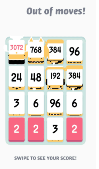
Many players would recognize 2048, the hit indie game created by Gabriele Cirulli over 10 years ago. In this game, players slide tiles on a 4×4 grid. When two tiles of the same number touch, they combine in powers of two (2 and 2 make 4, 4 and 4 make 8, and so on.). Players would try to create the largest tiles possible in order to achieve the 2048 tile (or much, much higher) before the board was filled and they were left unable to move.

Do you notice any similarities in the following image?

Much lesser known was the game that inspired it — Threes — likely due to it being harder right out of the gate. The rules of Threes are mostly the same as 2048 — with a few key differences.
- Tiles start at 1, 2, 3, 6, 12… (then continuing to double) instead of 2, 4, 8, 16, 32.
- Two different digits (1 and 2) are required to make 3.
- Tiles only slide one space when moved.
- Players get information about the next tile to spawn, with an equal probability of being a 1, 2, or 3, and a rarer chance of being an unknown bonus high-value tile.
- There are also far more intricacies to the spawning mechanism that can be utilized by the player, but they are too verbose to discuss here.
By far, the most interesting gameplay difference is the lowest merge: Instead of combining 2 and 2 to make 4, players must instead combine 1 and 2 to make 3. Marginal enough?
The problem is, instead of being able to reliably merge any existing 2s with a future 2 (which 2048 will almost always provide you with), you might get a lot of 2s that clutter the board without any 1s, or vice versa. The game does have a system in place to ensure that the difference between 1s and 2s is at most four, but this means players can lose up to four tiles of space instead of one.
The one and only compensation is that the locations where tiles spawn are more predictable and can be influenced by clever play. However, unless you give it special attention, new tiles tend to spawn in the worst possible positions, particularly when you move your big tile out of a corner.
Vollmer spent months on this trying to ensure a simple algorithm couldn’t easily beat his game, unlike pre-endgame 2048. He succeeded.
The world’s hardest game?
The two hardest Threes achievements (not counting the uncompleted community achievements) are as follows:
- Create a 6144-tile. The vast majority of players haven’t gotten close, and the best players can only reach it around half the time. (The equivalent in the game 2048 is 16384.)
- Create a 12288-tile. The final tile that can be mathematically reached is 12288, even with absolutely perfect play, barring extreme RNG manipulation. (The 2048 equivalent is 32768.) Regardless, the game automatically ends once this tile is created.
So, how difficult is it to achieve these?
Let’s look at the Challenge Enthusiasts site, which compiles difficult achievements from some 2,000 single-player games and tiers them. It’s not perfect, as many of these games come from extremely different genres, but it should give some sense of comparison. Higher-numbered tiers are more difficult.
The hardest Dark Souls game is Tier 2, also shared with DELTARUNE, which has an achievement for no-hitting the Chapter 3 final boss.

Touhou is a shoot-em-up genre where you have to dodge hundreds, if not thousands, of bullets — clearing such a game is typically around Tiers 3–4. Games in the series without a perfect run achievement are only Tier 3. However, there are multiple fangames with comparable difficulty that do require a perfect run for completion around Tier 4. While I could argue why I think those are underrated, the following picture should get the point across.

Celeste’s Farewell Golden is in Tier 5. Below is one of the easier sections, which I have cherry-picked because it looks scary.

Which would win? Is it the 20 to 40 minutes of flawless dodging or platforming with no mistakes, or the cute minimalistic sliding numbers game?
The answer is, of course, the Cute Minimalistic Sliding Numbers Game, which is Tier 6 out of 7.

Reaching 6144 is quite difficult already, as there are fewer than 100 confirmed clears. Most players don’t get anywhere close.
Fewer than 10 people have achieved a confirmed 12288, and that’s not for lack of players — even the best players have about a 5% success rate, or even less. There’s even a community strategy guide dedicated to reaching 6144, which has close to zero information on 12288.
Let’s see if RL can match them.
Why I used PufferLib
Previous RL attempts
A previous attempt to design my own RL environment for Connect 4 in a university project ended in disaster: An agent wouldn’t block wins-in-one about a fourth of the time, for a few reasons.
- Deep Q-Networks performed poorly on complex two player games. Representing a deep minimax game tree, even a simple one, is substantially harder than the Atari games of old which DQN performed well on. When I switched to using stable-baseline’s PPO wrapper, I instantly got good enough results that could take games off intermediate players like myself if they got complacent.
- Running and simulating games took forever. We were using Python, and as everyone knows, unoptimized Python is like 50 times slower than C++. As is typical of machine learning, vastly more time was spent tweaking hyperparameters and debugging than actually training the final model, and this made the programming process very painful.
- Implementing everything from scratch (including the environment, DQN, the Replay Buffer, etc.) made for extremely difficult debugging.
It’s not like the model learned nothing; it knew to prioritize the center, and it would spot wins in one enough of the time. But it was constantly outperformed by a simple, 2-depth heuristic search.
The blowfish
With a few more years of computer science experience under my belt, I decided I was going to give RL another shot. A friend recommended PufferLib, an open-source library that uses PPO. PufferLib provides the following:
- Fast vectorized environments. Running environments in parallel is much more cache efficient. Some projects even demonstrate a 10x speed increase, though PufferLib has many other optimizations that make it far faster.
- Simplified environment training. The train loop is just a 1000-line script with minimal Object-Oriented structures. It’s not necessary to understand most of the codebase to use or process it.
- Automatic hyperparameter sweeps using PROTEIN (an improved variant of CARBS). The assurance that a set of hyperparameters are close enough to optimal is such a burden-reliever, as you don’t have to manually train some 20 models to confirm that gamma is 0.995 or 0.999 (this can make quite a difference).
Most importantly, it has achieved prior success in many environments, many of which can be utterly complex. It even beat Pokemon Red, a comparatively massive undertaking.

Apparently, the LLM Gemini beat Pokemon Red shortly after David Rubinstein and his team did with PufferLib. Despite having internet access to all Pokemon statistics, map information, and a wealth of strategy guides, Gemini still required a lot more handholding. That’s another win for RL.
It didn’t take much persuasion for me to switch to PufferLib after reading that. I started toying with Target, a baseline environment featuring an agent moving along a large grid onto a randomly placed green cell. I added 20 red cells (also randomly placed) which penalized the agent if it touched them, and the model learned to avoid them surprisingly well.

So what’s the next step? Well, there was already a 2048 environment I could build on, so why not see how well a model could utilize the additional information and constraints that Threes provides to survive the much harsher early and middlegame?
How the model works
Designing the game environment
Creating the environment was mostly smooth sailing, once I had learned the rules for all the spawning and movement mechanics. There were a few options I could have chosen, though:
First, I initially used one-hot encoding for the board, meaning the model perceives each different piece value as an entirely different object rather than ‘three times the previous piece.’ Otherwise, the model would likely learn a false numerical relationship between pieces, and would especially struggle to handle the fact that some numbers were way higher than others. A linear model with a few activation functions would be required to distinguish 6144 and 3072, but also 6 and 3.
I later replaced this with embeddings, with dimension size 8. However, both functioned similarly enough and neither were the main performance bottleneck — the large fully connected layers.
How the model learns
Secondly, the model’s reward function had to be well-chosen. The reward function is the only factor the model uses to determine how successful a game was — and how it would learn. The main concern was that Threes was an exponential game, in that scores were often sums of values of the form 3^n.
Neural networks are essentially built from layered linear functions with nonlinear activations, so they tend to approximate smooth or piecewise patterns more easily than exponential ones. It might as well try modelling y=e^x with three line segments. You’ll find that models would often resort to casework to get around this problem. So, it was in my interest to choose a reward function that didn’t exponentially explode.
There were quite a few additional options for the reward function that weren’t exponential:
- Game length. The longer you survive, the cleaner your board must have been to survive.
- Number of merges. Not only does this have direct correlation with game length, but it incentivizes merging large tiles together.
The authors of the 2048 environment had already chosen a decent reward function, which was the number of merges, multiplied by how many ‘layers’ deep the piece was. Given their success, I saw no reason not to use it as well.
The final score in Threes is also entirely computed at the end, though the model never sees it and it’s only useful as a human evaluation metric. I ended up breaking it up into tinier pieces that added score upon every merge. However, in the end, the final score would be equal to the actual score.
Actor-Critic architecture explained
Third is the model itself. I didn’t deviate much from the 2048 structure outside of layer sizes, as it passed most of my checks for what a decent actor-critic network should resemble. It looks like this:

An AC network comprises an Actor and a Critic. Both receive the state of the board. The Critic assigns an approximated value to the board position, and the Actor chooses the best move in the current position, using the Critic’s estimated values to improve its behavior. Note that the Critic’s value is different from the reward function, as it tries to estimate the sum of all future rewards instead of just the current or final reward value. We simply do not have access to this, so we need some function to estimate it.
Empirically, keeping the Actor and Critic somewhat separate has been shown to give better results, as the task of evaluating the current board state and choosing the right action are different enough. While they’re not fully separate here, they have two separate FC layers which allows them to specialize.
The LSTM layer allows the model to learn relationships between its state and its previous states. It also adds minimal computation overhead. While there technically is zero benefit to knowing board history, it could allow the network to learn the effects of each action, as they progress the board from its current to its next state. There is, however, an additional cost to the LSTM layer, as we shall see later.
Training / Hyperparameter Optimizations
Why tuning matters
Enough following the 2048 architecture. Training, unfortunately, does not spare me the luxury of following along and deviating from the template whenever necessary.
PufferLib’s implemented PPO variant has far too many hyperparameters, probably some 25 to 40 in total. If I had a mortal enemy who could adjust just one of these numbers to mess with me, the results vary from ‘this model now takes twice as long to train’ to ‘the model is lobotomized and incapable of learning anything,’ with the majority of situations being the latter.
Apparently, even those studying RL are not immune to brainrot. This questionable number of timesteps was part of the default parameters from 2048.

Getting the Learning Rate right
The primary hyperparameters that I found worth adjusting were the following:
1. Learning rate (LR). Basically, imagine the model as a ball rolling around a mountain ridge, and where we’re trying to bring it to the lowest valley. (It even has some form of momentum, thanks to the Adam optimizer). If there’s a slope, it’ll take the quickest path down. Learning rate is the speed at which it descends.

If the LR is too low, the ball would take forever to go anywhere. For instance, if LR is 10 times lower, performance would be theoretically close to 10 times slower.
If the LR is too high, the ball would overshoot the hole. If the LR rate is really high, the ball flies off into the stratosphere. Obviously, this is terrible.
This creates what I affectionately refer to as NaN hell, where the model is effectively dead and all your aforementioned training is wasted.
As the game gets harder, the ball must fit through more and more precise gaps, so LR must be lowered accordingly. This (among other stability reasons) is why learning rate annealing is all but required.

Additionally, there are many ‘ledges’, or local minimums where the model can stop at. If our learning rate or PPO clipping values are too low, the model could end up permanently at a local minimum instead of near the bottom.
The other key hyperparameters
2. Gamma. I said earlier that the reward function is a sum of future rewards. This isn’t entirely true; the model weights future rewards more heavily when gamma is high, and vice versa. Too low of a gamma will create a ‘greedy’ model that will not think long term, and too high of a gamma leads to overfitting and other consequences. It’s basically just a geometric series, where the reward n steps ahead is multiplied by gamma raised to the nth power.

3. Total timesteps. This is how many steps the model trains for. Not particularly surprising.
4. Model size (input_size and hidden_size). The right-sized model can theoretically learn more, and do so faster. Too large, and it’s too slow for both learning and execution. Too small, and it won’t learn anything beyond the basics, or anything at all. I found that the model can play decently well with a size of 256, but I used a size of 1024 to push the success rate higher.
I did around 150 experiments adjusting these values under different conditions. Some of my observations (as well as graphs) are in the latter section.
Hyperparameter sweeps
As I’ve elaborated on before, it is likely that far more time is spent setting hyperparameters or dealing with issues than training the final model. After all, the difference between good hyperparameters and passable ones could mean the difference between success and failure.
Unfortunately, to my limited knowledge, there is no way to determine which hyperparameters are decent without some amount of trial and error, and this includes training a whole slew of models ranging from effective to useless. For each new model we train, we have to launch another training run from start to finish.
The old-fashioned technique for hyperparameter sweeps is called grid search. If there are more than 3 to 4 hyperparameters, you freeze the excess at reasonable, specific values — which unfortunately requires RL experience and domain knowledge. Then, you assign each hyperparameter you are adjusting a list of potential values — which also requires RL experience and domain knowledge. Then, you iterate through all possibilities, and the list grows exponentially large for each hyperparameter you run through the sweep. But remember, if any of your other hyperparameters are set too far incorrectly, training might be near-impossible.
Imagine you’re testing 5 values for just learning rate, gamma, and hidden size. That’s 125 models, and odds are, 100 of them are going to be terrible.

There are a few improvements we can do, of course. The first is simply killing off runs that are clearly dead in the water before they can fully complete. The second is using PufferLib’s PROTEIN sweeps, which uses a variant of local search to find the Pareto front.
What this means is that PROTEIN attempts to find the ideal model parameters for various possible training durations (or other costs) by trying individual points. Later on, it focuses more on points that perform better, meaning that we can afford to have much more hyperparameters being swept, which is crucial for PPO. PufferLib projects can have up to 30 to 50 hyperparameters, which would be completely impossible to grid search.
Even still, training like this would be a substantially difficult task that would take hours to train, and I didn’t have the compute to multiply that for each sweep. Instead, I stopped each sweep as they approached 5 to 10 minutes of runtime, allowing me to get around a hundred trial runs in. Of course, the hyperparameters that perform well at the start will give performance nowhere near the hyperparameters that perform best in the long run, but it’s at least something — and I can always drop the learning rate later.
Outcomes
Early results
The goal of the project was to get as close to the 6144-tile as possible, so I judged performance by the size of the largest tile, divided by 6144. While consistent 6144s are not realistically possible, I would be happy if I could be fairly consistent reaching 3072 and hit 6144 every now and then.
The initial results after training for 500 million steps with LR=0.04 looked like this:

The model was often bouncing between max tiles of 786 and 1536 in the first iteration, which was already pretty impressive. However, it would quickly plateau. I would resume from a checkpoint and then halve the learning rate, which allowed it to go further but at decreased progress. I would repeat this every time I saw the model plateau, and the model would advance a bit further every time.
Midway through training, I wondered what would happen if I ran another hyperparameter sweep, except centered around fine-tuning a checkpoint model. My main speculation was that the model would ‘freeze itself’ at first to avoid messing itself up, but I was hoping that it would learn something later in the process.
This little side tangent used quite a bunch of compute time just for the chosen hyperparameters to provide worse results than the first ones, though it was still learning — albeit very slowly.
In pink, the model with the initial hyperparameters. In brown, the model with the later set. Initial ones performed marginally better.

Final results
As for the final model, I was able to reach a final performance of 0.55, meaning it was able to make 3072-tiles most of the time. It could also make 6144-tiles with decent frequency.

==================================================
Results from 200 games:
==================================================
Highest Tile Count Percentage
--------------------------------------------------
6144 33 16.5%
3072 129 64.5%
1536 32 16.0%
768 6 3.0%
==================================================
And it was able to hit 12288-tiles in training. This is sufficiently rare, occurring at a probability of 0.065% (roughly 1 in 1500 times).
Conclusion
The model was a success, playing Threes better than all but the best human players (again, only some hundred players have confirmed 6144-tiles).
I didn’t really have the expectation of beating the best human. Nor was I beating the best Threes AI, which got a 6144-rate of 20%, which used a form of search called Expectimax.
But my model was much, much faster. And with its speed, it was able to learn to be able to hit 12288 a fair amount of the time, at least in training runs, which no other AI to my knowledge has done.
I also learned a lot from the process, becoming more familiar with each of the following:
- The PufferLib library, of course, as well as NumPy/Torch (more prevalent when running experiments with ConvNets and Embeddings).
- C Programming — PufferLib uses C-wrappers in order to make training as fast as it is. While I have been fairly acclimated to C++ for a while, it’s been a while since I’ve done anything without the C++ standard library.
My main takeaways
- Vectorization and running numerous environments in parallel is absolutely critical in RL. Models take a lot more iterations to learn than we do. I do find it impressive that humans are a lot better at learning with far less experience.
- If all else is equal, simple models are the best, as you have less moving parts to finagle and spend time and money fixing. I learned this while briefly toying with CNNs, as well as cyclical learning rate annealing. While I had good reason to believe they would perform better, they only barely matched the performance of the models without them while creating additional complexity. Simple is also a lot easier to implement.
- Deal with the tightest bottleneck first, and avoid premature optimization. Prematurely optimizing other things could always be done later. I learned this the hard way while trying to make my environment as fast as possible — the bottleneck, I later learned, was the model, and what I did had little effect. Later, I tried to decrease the input size of the board, because I was afraid that embeddings or one-hot encodings were too large: I had entirely forgotten that the fully connected parts of the model were much larger and therefore more time-consuming. Better to just focus down the narrowest chokepoint first, and then adjust things later in the process.
There’s also a bit more to be done, were I to return to this in the future. I could attempt model distillation in order to allow for faster evaluations and faster sweeps, since I speculate most of the massive parameter count is excessive. I also theorize I could use my model (with a bit of fine-tuning) with Monte-Carlo Tree Search (MCTS), which would almost certainly improve the success rate drastically at the cost of time. I have always wondered what the optimal success rates are, and maybe I’ll be able to get very, very close to them with MCTS.


Be First to Comment